

commonchaffinch @commonchaffinch@qoto.org
English/中文
Environmental scientist looking at global ecohydrological change using data analysis and modeling tools.
Joined May 2022
commonchaffinch
boosted

A friend got this as a #Springer #journal #editor. I expect it will work about as well as #plagiarism detection #software generally does. Maybe worse, since journal writing in particular is known for forcing human* authors into a very mechanical #writing #style. There may be nothing easier to mimic for #ChatGPT et al.
*Presumably.
commonchaffinch
boosted

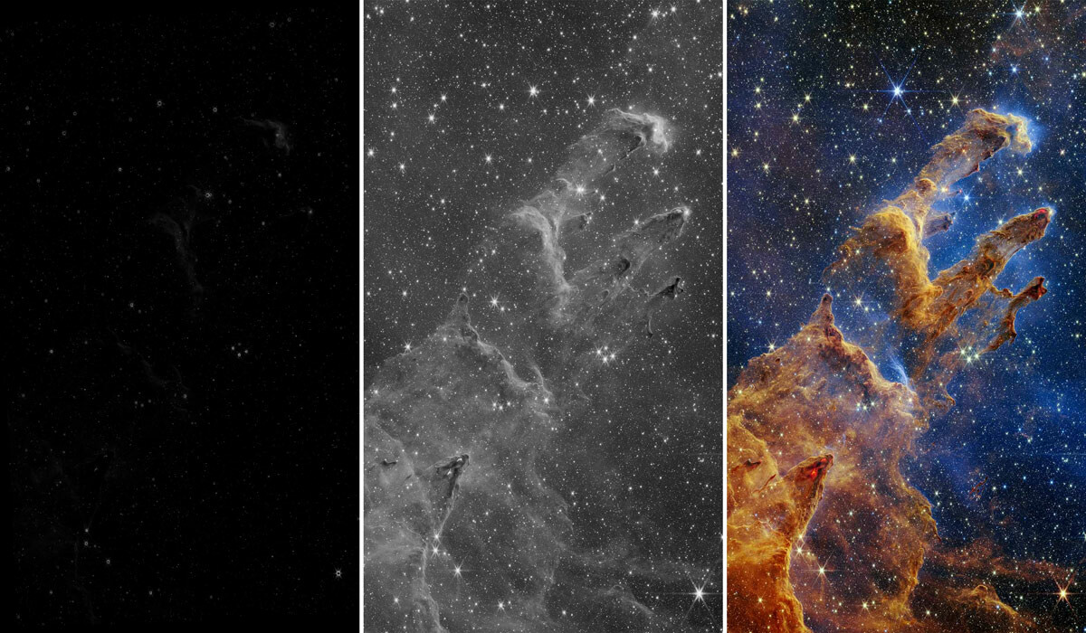
It turns out that while #JWST is sort of like your phone’s camera, making images with a 10 billion dollar telescope designed for science observations is a little more tricky than point and shoot.
More about the image processing process:
https://webbtelescope.org/contents/articles/how-are-webbs-full-color-images-made
In the past couple days, I had to delineate a watershed using the PCRaster tool for some hydrological modeling work. Despite the excellent tutorial of https://github.com/jvdkwast/PCRasterTutorials/tree/main/PCRasterCatchmentDelineation, there were several pitfalls that took me a long while to figure out.
The first is, how do I know what x-y coordinates to put into "location.txt"? I only know the latitude and longitude of my stream gauge, but they did not work when I tried putting them in. It turns out the x-y coordinates are the coordinates of this stream gauge in the projected coordinate system of the flow direction (ldd) map. As such, the easiest way to approach the problem seems to be to use the QGIS PCRaster plugin. First, import the digital elevation map into QGIS, reproject it into a projected coordinate system, and set the layer's coordinate system to be the same as the digital elevation map. Second, calculate the ldd map using the PCRaster plugin's `lddcreate` command, so that the ldd map has the same projected coordinate system. Third, load the text file containing the lat-lon of the stream gauge as a map layer. QGIS automatically does the conversion, so that the gauge is shown in its correct position in the projected coordinate system. Fourth, calculate the stream order from the ldd map using the PCRaster plugin's `streamorder` command and check if the gauge is actually located in the correct stream. This is important because the lat-lon coordinates and the digital elevation maps are not entirely accurate, often causing the gauge to be outside the stream implied by the ldd map. If the gauge is outside, find the nearest in-stream pixel that seems to make sense. Placing the curser on top of the nearest in-stream pixel finally makes QGIS show the desired x-y coordinates in its status bar.
The second is, how to install the PCRaster plugin in QGIS? The plugin does not work on its own. Instead, one must install PCRaster in the same Python environment as QGIS accesses. In the end, I had to create a new conda environment and install PCRaster and QGIS both from the `conda-forge` channel. Moreover, the default `conda create -n ` command now pulls Python 3.11, but this Python version does not support compatible PCRaster and QGIS releases. I set the Python version to 3.9 to finally make things work.
The third is, why is my delineated catchment area incorrect? My stream gauge is on a major river so I know it must cover a large catchment area. Yet I got a zero-sized catchment at my first try. It turned out that in running the `lddcreate` command in PCRaster plugin, one must remove pits - pixels that draw flow from all directions and do not let water flow out - that do not make sense. One can set thresholds in the "Outflow depth", "Core area", "Core volume", and "Catchment precipitation" in the options of the `lddcreate` command to remove pits that are too shallow or too small. The default thresholds were too small for me, and as a result, the pits broke up my major river into many small ones in the stream order map created from the ldd map. After I set the Core area to be five times the default 9999999 (map units, for me it was meters), my delineated catchment finally made sense.
commonchaffinch
boosted

Nuclear #fusion will not only come too late to help solve the #climatecrisis. Even in the long run it will not be the unlimited energy source that some are dreaming of. The reason is basic physics, and anyone can do the back-of-envelope calculation. 🧵1/
commonchaffinch
boosted

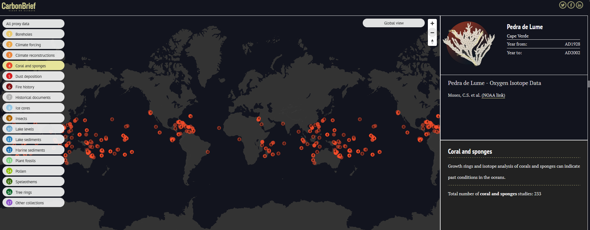
I really love this @carbonbrief compilation led by @hausfath (i believe): https://interactive.carbonbrief.org/how-proxy-data-reveals-climate-of-earths-distant-past/. Really useful to the public and climate scientists like me who need help in compiling data!
commonchaffinch
boosted

I’m seeing more and more #earthscience people joining mastodon everyday. If you are not on the list linked below, please ask to be added by contacting Chris Rowan at @allochthonous The list allows newcomers to quickly follow you by exporting the list and importing it under the Import and Export option under Settings. Thank you, Chris!
commonchaffinch
boosted

#FollowFriday #Climate scientists and scholars
@Ruth_Mottram
@gwagner
@lcooley@weburbanists.com
@wolfgangcramer
@rahmstorf
@MichaelEMann
@climatedynamics
@hausfath
@DewiLeBars
@SoniaSeneviratne
@benmsanderson
@roelof
@natalyagomez
@ed_hawkins
@hereidk
@agrinsted
@petergleick
@julesberry
@mtobis
@jdannan
@Co2ley
@marcyrockman
@richardtol
@pfriedling
@pdemenocal
@davidho
@coralsncaves
@Val_Mueller_ASU
@meinshausen
@aldanacohen
@DoctorVive
@edwardcarr
commonchaffinch
boosted

The good agreement with simple physical theories confirms previous predictions that, as the globe warms, TCs will become more intense and destructive.
TCs will also increase their destructiveness because: 1) they are riding on a higher sea level, increasing coastal inundation, 2) rainfall is predicted to increase with warming.
For a good discussion of the issues, see this page from NOAA GFDL: https://www.gfdl.noaa.gov/global-warming-and-hurricanes/
#misc_thoughts
#ecology
#global_environmental_change
I always have this doubt that a lot of large-scale studies on how the terrestrial vegetation and carbon cycle respond to climate change can be "wrong". These studies often used relatively simple statistical tools (regression, basic machine learning, structural equation modeling) to investigate a small slice (from what I see, generally < 7 variables) of a huge system. The fitted relationships inevitably miss many intermediate causal relationships and all the influences from the not-included variables. As a result, the fitted relationships may be unable to reliably project future changes. Although land surface model is always available as an alternative tool, they have their own problems because their structures are less flexible and typically lag behind current experimental understanding and the parameters are not always well-calibrated.
Wonder if there are studies that already address my doubt?
一个试验。
最近做的项目需要训练~40k行17列的数据。Predictand的standard deviation在0.5左右。
用XGBoost RMSE在0.28左右,代价是50000 boosting rounds @ lr = 0.001。如果把learning rate调成0.0001看上去还能更好,但是需要的boosting rounds已经超过可行范围了。使用一个32 core, 64 GB的CPU node,训练时间比使用一个NVIDIA® K80 GPU还短一点。也可能是我GPU没有调对。
用同样的maximum tree depth训练Random Forest只需要500个tree,训练时间是XGBoost的三分之一,RMSE涨到了0.35,把tree增加到50000也只能微乎其微地降低RMSE。
In 2022, Kimberly A. Novick from the O'Neill School of Public and Environmental Affairs in Indiana University—Bloomington and coauthors discussed opportunities for ecosystem observations to inform nature based carbon sequestration solutions (NbCS).
The study "outline[s] steps for creating robust NbCS assessments at both local to regional scales that are informed by ecosystem-scale observations, and which consider concurrent biophysical impacts, future climate feedbacks, and the need for equitable and inclusive NbCS implementation strategies."
The study envisions the creation of "gold-standard datasets" that represent a full suite of carbon stock and flux measurements, including NbCS "treatments", baseline controls, and information about historical land use. The sources of the datasets include flux tower, survey, remote sensing, and models.
Opportunities:
(1) Flux tower data with limited spatial fingerprint may be combined with broader tree survey data.
(2) We do not have spatially explicit maps of cropland NbCS mitigation potentials, and do not know where climate conditions may favor or disfavor the use of cover crops to enhance carbon uptake.
(3) Coastal sequestration in tidal wetlands and seagrass are promising opportunities (~25 Tg CO2e year-1). Flux towers can be used to analyze the impacts of optimizing NbCS in carbon uptake and sequestration.
(4) Next-generation remote sensing measurements include solar-induced fluorescence, column-averaged atmospheric CO2, instruments for sensing ecosystem water stress (ECOSTRESS), microwave data on canopy water content. Some of these are at scales that match individual farms. There are also drone-mounted instruments. These can be merged with flux tower data following past approach like machine learning, but for a specific region to produce more accurate regional baseline maps.
(5) Reduce uncertainty in ecosystem models. Price in the uncertainty into market systems. How does high resolution simulations improve results. Model-data assimulation for near term ecological forecasting and landscape scale model-data fusion.
(6) NbCS projects modify local water and energy cycles, which makes it necessary to consider potential negative consequences in these that consistitute trade-offs with the global climate benefit.
(7) Design and validation of new market structures and inclusivity of solutions.
Case study
(1) The benefit-cost trade off of establishing a flux tower site for monitoring NbCS project is calculated.
(2) A conceptual diagram for combining tree intentory, soil cares, static chambers, flux tower, and remote sensing to create project carbon grids for monitoring purpose.
When using matplotlib.colors.BoundaryNorm, the number of colors argument must match the number of colors in the colormap (256 by default). Otherwise, the normalized colors won't cover the whole range of the colormap.
libicui18n.so.58 is an ICU library image - International Components for Unicode.
commonchaffinch
boosted

I'm thinking about switching from google drive to dropbox, due to safety reasons (I don't want any suspicious AI spy on my files). Today I noticed the Hetzner Storage box and mountain duck.
Hetzner storage box offers 1TB network drive for 3.2 EUR per month, and mountain duck offers a way to mount that network drive on Windows, with a 39 USD one-time fee. The software is made in swiss.
Due to the god damn GFW in China, the speed can't go over 100KB/s without proxy. Thankfully, with my proxy server set up on the Hetzner FSN datacenter, the upload speed is faster than 4MB/s, which I think is the limit of my network. The download speed is also not bad: 8MB/s at the beginning, drop to 2MB/s, sometimes stuck at 2Mbps. Not sure who should be blamed for this, since there are too many participants involved: mountain duck, my transparent proxy, my network ISP, the proxy server on Hetzner, Hetzner storage box, I don't know. But with WebDAV, it supports random access, which means I can stream a video and scroll back and forth without waiting for the stupid client software to download the entire file (It's you, Google Drive Client).
The price is also the cheapest. Hetzner's price is equivalent to 38.16 USD per TB per year (BX11, with BX41, you get 24.246 USD per TB per year), while Google Drive (2TB annually) is 49.995 USD per TB per year, and dropbox (2TB annually) is 59.94 USD per TB per year. The proxy server is kind of required no matter which service I use, so that's not a big game changer.
I will try this configuration for a while. If I think it's good enough, that would be a great deal.
#杂感
似乎现在才渐渐开始理解使用已被证明的方法、可重复性、数据质量的重要性。文献最重要的部分往往是方法,概念不是真的,同一个概念可以对应不同的数学变量,而真正的现象体现在数学变量上。
To cope with memory limit when working on large netcdf datasets, `xarray.open_dataset(..., chunks = {'time': ...})` works, but rechunking the data after the read statement does not work.
Tests for my code must have 100% coverage, that is, make sure every line of the code is run at least once. This can be achieved by using coverage.py with tox.
The article also talks about preparing and uploading the package to PyPi using Poetry, pretty formatting using black, creating release tags on Github, CI/CD using Github Actions, and adding badges to README.md.
https://mathspp.com/blog/how-to-create-a-python-package-in-2022#a-simple-tox-configuration
I think people in science like people who explore and measure the external world.
#research_diary
#urban_heat_islands
I was plotting a generic map of daytime urban heat island intensity (UHII) today (left, color goes from slightly below 0 to 2.8 degrees). The map turned out to be vastly different from the previously reported spatial patterns, where the UHII clearly increases from the west to the east (right, from Fig. 1 of Zhao et al. 2014, DOI: 10.1038/nature13462).
Then I realized my variable was 2m air temperature, and their variable was land surface temperature. So I recalled another paper that showed the west-east divide in UHII for 2m air temperature (Fig. 3 of Zhao et al. 2018, DOI: 10.1088/1748-9326/aa9f73). As expected, there was no east-west divide in the UHII shown in the barplot.
Are the well-known evaporative and/or convective cooling effects on UHII in the west only applicable to the land surface temperature?
English/中文
Environmental scientist looking at global ecohydrological change using data analysis and modeling tools.
Joined May 2022
